Load Dissipation

As promised, here is the second part of this two-part blog series. In the first section, I discussed the standard live load design vehicles and presented the design methodology of these vehicles. In the second part of this series, I will discuss how the live load dissipates, and how to determine the live load pressure at various cover depths for both standard highway loading and construction vehicles. 

You may be asking yourself, how is a live load pressure determined at various cover depths? The answer may be easier than you would expect. The pressure is determined by taking the live load at the surface divided by the distributed tire load at “x” depth. There are however multiple methods to determine how the live load is dissipated into the soil, which are explained below.

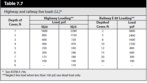
If you remember from the first series, I had included Table 7.7 from the NCSPA book with specific live load pressures at various cover depths. This table is attached again below and can be described as the traditional method. For this table, the pressures are based on load application through a 12” thick pavement with an area of 10 square feet, and pressure distribution through the soil in accordance with elastic theory (Boussinesq method).

Furthermore, there are alternate methods for the dissipation of live load pressure based on various load distribution slopes. The NCSPA Design Manual publishes using a load distribution slope of ½ to 1 (horizontal to vertical), while section 6.4 of the AASHTO Standard Specification for Highway Bridges references using a 0.875 to 1 load distribution. An easier way to think about this is to assume the load is being distributed over the base of a truncated prism, with the side slopes of 1 vertical and 0.5-0.875 (depending on methodology) horizontal. Using a ½ to 1 load distribution slope is the most conservative, and is recommended for use on heavier construction loading vehicles. For heights of covers under 3’, there are additional impact factors that should be included, as detailed by AASHTO.

For non-standard vehicles, several factors need to be known to determine the live load pressure: weight of the vehicle, the number of wheels/axles, axle spacing, and the contact area of the tire. Each of these can be found in the vehicle manufacturer’s specifications. For standard highway vehicles, each of these variables are spelled out in AASHTO. Per AASHTO, the tire contact area shall be assumed to be a rectangle whose width is 20” and length is 10”. It should be noted that the tire pressure is assumed to be uniformly distributed over the contact area for both standard and non-standard vehicles.

I will go through a quick example for both an HS-20 truck using a 0.875 to 1 load distribution, and a construction loading vehicle (CAT777D Articulated Truck) using a ½ to 1 load distribution at 5’ cover.

To recap, an HS-20 vehicle has a 32,000 pound axle (two - 16,000 pound wheel groups) and a tire contact area of 10” x 20” (0.83’ x 1.67’). Using a 0.875 to 1 load distribution would cause the length to be equal to 0.83’ + 0.875H + 0.875H (which can be simplified to 0.83’ + 1.75H). Similarly, the width can be simplified to 1.67’ + 1.75H. Below is an isometric image to further clarify this dissipation.

Using these aforementioned equations at 5’ of cover will yield a distributed length of 9.58’ and a width of 10.42’. To determine the live load pressure at 5’, you would take the 16,000 pound wheel group and divide it by your distributed load area (9.58’ length x 10.42’ width) to get a live load pressure of 160 psf. From comparing this to the above table, you can see this approach produces a slightly smaller number than the traditional method at 5’ of cover.

Now, let’s run the same exercise for a CAT777D Off-Highway Truck. This vehicle consists of two axles, with the back axle containing tandem wheels. Looking through their specifications, the total operating weight is 360,143 pounds with 67% of the weight on the back axle (241,300 pounds, or 120,650 pounds per back wheel group). The standard tires are 27.00-R49 (E4) tires. This tire has a gross contact area of 707 square inches, a width of 29.8 inches (2.48’) and length of 23.7 inches (1.97’)—the tandem tires would have a combined with of 4.96’, with a length of 1.97’. The axle spacing is 15’.

As earlier discussed, for construction loading applications we would recommend using a load distribution of ½” to 1. Knowing this, the equation for the length would be 1.97’ + 0.5H +0.5H (simplified to 1.97’ + H), and the equation for the width would be 4.96’ + H. At 5’ of cover, the distributed length would be 6.97’ and distributed width would be 9.96’. Dividing the 120,650 pound wheel group by this distributed area will equate to a live load pressure of ~1,740 psf at 5’ of cover.

For vehicles with lesser axle spacing, the distributed load tire areas may overlap. For these cases, you can consider the weight of all interacting wheels and divide it over the distributed area for each of these interacting wheels to determine the appropriate live load pressure.

Hopefully that provides some insight into how live loads disspate. Of course, feel free to reach out to me if you have further questions!